Simulating Quantum Dynamics: From Neutral Atoms to Noise Modeling with Python

Introduction to the New Era of Python Quantum Simulation

The landscape of quantum computing is undergoing a paradigm shift. While gate-based superconducting circuits have long dominated the headlines, the rise of neutral atom quantum computing—exemplified by platforms like QuEra—has introduced new possibilities for analog Hamiltonian simulation. For Python developers and researchers, this evolution demands a deeper understanding of the ecosystem. We are moving beyond simple circuit construction into the realm of complex dynamics, stochastic collapse models, and noise engineering. With Qiskit news constantly breaking and libraries like QuTiP providing robust backends, Python remains the undisputed lingua franca of quantum mechanics.

However, simulating quantum systems is computationally expensive. As we scale to larger qubit counts (or atom arrays), the efficiency of our Python code becomes critical. This is where the broader Python ecosystem intersects with quantum mechanics. Innovations such as GIL removal and free threading in upcoming Python versions, along with the performance boosts from Rust Python integrations, are set to revolutionize how we handle the massive state vectors required for n-qubit simulations. Whether you are exploring topological phases using Fibonacci geometries or modeling decoherence in biological quantum theories, the modern Python stack offers the tools necessary to bridge theory and reality.

In this article, we will explore how to architect high-performance quantum simulations. We will focus on neutral atom dynamics, noise modeling using the Lindblad master equation, and how to leverage modern tooling—from Polars dataframe for result analysis to Uv installer for dependency management—to build a production-grade quantum laboratory on your local machine.

Section 1: Modeling Hamiltonian Dynamics with QuTiP

To simulate neutral atoms or any continuous-variable quantum system, we often step away from the discrete gate model and look at the Hamiltonian evolution directly. The Quantum Toolbox in Python (QuTiP) is the industry standard for this. It allows us to solve the Schrödinger equation and the Lindblad master equation for open quantum systems.

In the context of neutral atoms, we are often interested in the Rydberg blockade mechanism. However, before simulating a full array, one must understand how to model a single driven atom subject to noise. This is akin to the foundational work required before scaling to cloud platforms like Aquila.

Below is an example of setting up a time-dependent Hamiltonian simulation. This setup is crucial for implementing pulse-level control, where the “gates” are actually continuous analog pulses.

import numpy as np
import qutip as qt
import matplotlib.pyplot as plt

def simulate_driven_atom():
    """
    Simulates a 2-level atom driven by a time-dependent field 
    with dissipation (spontaneous emission).
    """
    # Define the 2-level system (Ground |g> and Rydberg |r>)
    psi0 = qt.basis(2, 0)  # Start in ground state
    a = qt.destroy(2)      # Lowering operator
    
    # Hamiltonian components
    H0 = 0 * qt.sigmaz()   # Frame rotation (simplified)
    H1 = qt.sigmax()       # Driving term (Rabi flopping)
    
    # Time-dependent coefficient for the driving field (Gaussian pulse)
    def rabi_pulse(t, args):
        A = args['A']      # Amplitude
        sigma = args['sigma']
        mu = args['mu']
        return A * np.exp(-(t - mu)**2 / (2 * sigma**2))

    # Construct the Hamiltonian: H = H0 + f(t)*H1
    H = [H0, [H1, rabi_pulse]]
    
    # Collapse operators describing noise (spontaneous emission)
    # Rate of decay gamma
    gamma = 0.05
    c_ops = [np.sqrt(gamma) * a]
    
    # Time vector
    tlist = np.linspace(0, 20, 500)
    args = {'A': 5.0 * np.pi, 'sigma': 2.0, 'mu': 10.0}
    
    # Solve Master Equation
    result = qt.mesolve(H, psi0, tlist, c_ops, e_ops=[a.dag()*a], args=args)
    
    return tlist, result.expect[0]

# Execute simulation
times, excitation_prob = simulate_driven_atom()
print(f"Max excitation probability: {max(excitation_prob):.4f}")

In this example, we utilize NumPy news-worthy vectorization to handle time arrays efficiently. The `mesolve` function is the workhorse here. It solves the differential equations governing the system’s density matrix. When dealing with theories like Orch-OR or other collapse models, one might switch from `mesolve` (Master Equation) to `mcsolve` (Monte Carlo Wavefunction), which simulates individual quantum trajectories and stochastic collapses.

For researchers interested in Python automation, this script can be wrapped in a function and run across varying parameters (like pulse amplitude or decay rates) to map out the “stability zones” of the quantum operation.

Section 2: Scaling to Neutral Atom Arrays and Geometry

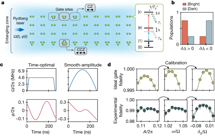
The true power of neutral atom platforms lies in the ability to arrange qubits in arbitrary 2D and 3D geometries. This allows for the simulation of topological phases of matter, such as those found in Fibonacci anyon models. While QuTiP handles the math, we often need specific frameworks to define the register layout and pulse schedules meant for hardware execution.

When simulating n-qubit systems, the state space grows exponentially ($2^n$). To handle this in Python without crashing your memory, you need efficient state representation. Libraries like Pulser allow you to define these geometries and export them for simulation or execution on hardware.

Here, we will define a geometric arrangement of atoms. We will use a Fibonacci spiral pattern as a nod to topological quantum computing concepts. This example demonstrates how to prepare a register that could theoretically be sent to a cloud backend.

import numpy as np
from dataclasses import dataclass
from typing import List, Tuple

# Utilizing Type Hints for better code quality and MyPy updates compatibility
@dataclass
class AtomRegister:
    coordinates: List[Tuple[float, float]]
    
    def to_array(self) -> np.ndarray:
        return np.array(self.coordinates)

def generate_fibonacci_spiral(num_atoms: int, scaling: float = 5.0) -> AtomRegister:
    """
    Generates atom coordinates in a Fibonacci spiral pattern.
    Useful for exploring isotropic interactions in neutral atom arrays.
    """
    phi = (1 + np.sqrt(5)) / 2  # Golden ratio
    coords = []
    
    for i in range(num_atoms):
        # Radius increases with square root of index to maintain density
        r = scaling * np.sqrt(i)
        theta = 2 * np.pi * i / phi**2
        
        x = r * np.cos(theta)
        y = r * np.sin(theta)
        coords.append((x, y))
        
    return AtomRegister(coordinates=coords)

# Generate a 20-qubit register
register = generate_fibonacci_spiral(num_atoms=20)
atom_locs = register.to_array()

# Example: Calculate pairwise distances (crucial for Rydberg blockade interaction)
# Using efficient broadcasting (NumPy)
diffs = atom_locs[:, np.newaxis, :] - atom_locs[np.newaxis, :, :]
distances = np.sqrt(np.sum(diffs**2, axis=-1))

print(f"Generated {len(atom_locs)} atoms in a Fibonacci spiral.")
print(f"Nearest neighbor distance (approx): {np.min(distances[distances > 0]):.2f} um")

This code snippet highlights the importance of Type hints and clean data structures. With MyPy updates, strict typing helps prevent errors when constructing complex quantum registers. Furthermore, calculating the distance matrix is the first step in determining the Interaction Hamiltonian ($H_{int} = \sum \frac{C_6}{R_{ij}^6} n_i n_j$).

If you were to scale this simulation to hundreds of atoms, you would likely need to leverage JIT compilation tools. While standard Python is fast enough for setup, the actual evolution of a 50+ qubit system requires specialized tensor network libraries or integration with Mojo language or C++ backends.

Section 3: Advanced Noise Analysis and Data Processing

Real-world quantum systems are noisy. Whether it is thermal relaxation, dephasing, or control errors, a robust simulation must account for variance. In the context of advanced theories involving objective reduction or specific collapse times ($\tau \approx 500 \mu s$), we need to analyze the statistical variance of our measurement results.

Modern data processing in Python has evolved. Instead of relying solely on standard Pandas, we can use Polars dataframe for lightning-fast analysis of simulation results, especially when running multi-threaded noise testing. The following example demonstrates how to run a parallelized simulation of noisy evolution and analyze the variance using modern tools.

import concurrent.futures
import numpy as np
import polars as pl
from time import perf_counter

def single_shot_experiment(seed: int, collapse_rate: float) -> dict:
    """
    Simulates a single shot of a noisy quantum process with random outcome.
    In a real scenario, this would call a QuTiP mcsolve trajectory.
    """
    np.random.seed(seed)
    
    # Simulate a process with variance dependent on collapse rate
    # Simplified proxy for complex dynamics
    base_outcome = 0.5
    noise = np.random.normal(0, collapse_rate)
    result = base_outcome + noise
    
    # Clamp result to physical probability bounds [0, 1]
    final_measure = max(0.0, min(1.0, result))
    
    return {
        "seed": seed,
        "collapse_rate": collapse_rate,
        "measurement": final_measure,
        "is_coherent": final_measure > 0.8
    }

def run_parallel_noise_study(samples: int = 1000):
    """
    Uses ProcessPoolExecutor to bypass GIL for CPU-bound simulation tasks.
    """
    start_time = perf_counter()
    
    tasks = []
    # Varying collapse rates to see effect on variance
    rates = [0.01, 0.05, 0.1, 0.2]
    
    with concurrent.futures.ProcessPoolExecutor() as executor:
        for r in rates:
            for i in range(samples // len(rates)):
                # Create unique seeds
                seed = i + int(r * 10000)
                tasks.append(executor.submit(single_shot_experiment, seed, r))
    
    results = [t.result() for t in tasks]
    
    # Use Polars for high-performance data aggregation
    df = pl.DataFrame(results)
    
    # Group by collapse rate and calculate statistics
    stats = df.group_by("collapse_rate").agg([
        pl.col("measurement").mean().alias("mean_prob"),
        pl.col("measurement").var().alias("variance"),
        pl.col("measurement").max().alias("max_out")
    ]).sort("collapse_rate")
    
    duration = perf_counter() - start_time
    print(f"Simulation completed in {duration:.2f}s")
    print(stats)

if __name__ == "__main__":
    run_parallel_noise_study()

This section touches on Python testing methodologies. When building a simulator, you are essentially building a scientific instrument. You must verify that your noise models behave as expected. The use of `concurrent.futures` is a standard approach to parallelize tasks, but with Free threading on the horizon in Python 3.13+, this pattern will become even more efficient, allowing true parallelism without the overhead of multiprocessing.

Additionally, for those integrating this into a web dashboard, frameworks like FastAPI news or Litestar framework are excellent for serving these simulation results via API. You could even build a frontend using Reflex app or Flet ui to visualize the variance reconfiguration in real-time.

Section 4: Modernizing the Quantum Stack

To build a truly “comprehensive” quantum tool, one cannot ignore the software engineering aspect. The days of messy Jupyter notebooks as the final product are fading. We are moving towards robust, installable packages.

Dependency Management and Packaging

Managing the complex dependency tree of quantum libraries (QuTiP, NumPy, Scipy, Matplotlib) can be a nightmare. Modern tools like the Uv installer and Rye manager are replacing standard pip/venv workflows. They offer significantly faster resolution times and better lockfile management. If you are building a library to share, using Hatch build or PDM manager ensures your project adheres to modern standards (PEP 621).

Code Quality and Security

Quantum code deals with probabilistic outcomes, making bugs hard to spot. Static analysis is your best defense. Integrating Ruff linter (an extremely fast Python linter written in Rust) and Black formatter ensures code consistency. Furthermore, given the sensitive nature of some research, Python security is paramount. Tools like SonarLint python can catch code smells, while checking dependencies against PyPI safety databases helps prevent supply chain attacks—a growing concern in Malware analysis.

Integration with AI and Edge

The convergence of AI and Quantum is inevitable. LangChain updates and LlamaIndex news suggest that we can now use Local LLMs to interpret simulation results or even generate pulse sequences. Imagine an Edge AI agent running on a control server that automatically reconfigures the variance parameters of a simulation based on real-time feedback from a PyTorch news-worthy neural network. This is the future of “Orchestrated” quantum control.

Conclusion

Simulating quantum dynamics in Python has graduated from academic curiosity to engineering discipline. By combining the physics engines of QuTiP and Pulser with the software engineering rigor of modern Python—leveraging Rust Python tools, Polars dataframe, and advanced concurrency—we can build simulators that are not only accurate but also scalable. Whether you are investigating the theoretical underpinnings of consciousness via Orch-OR proxies or simply optimizing a Rydberg atom array for cloud deployment, the tools are at your fingertips.

As you move forward, keep an eye on MicroPython updates and CircuitPython news. As quantum control hardware becomes more embedded, the ability to run Python closer to the metal (or the atom) will become increasingly valuable. The future is hybrid, high-performance, and undeniably Pythonic.