Beyond Point Forecasts: The New Wave of Probabilistic Time Series Forecasting in Python
Introduction
In the world of data science, time series forecasting is a cornerstone, powering everything from inventory management and financial modeling to resource planning. For years, the standard approach has been point forecasting—predicting a single, most likely value for a future time point. While useful, this method has a critical flaw: it fails to communicate the inherent uncertainty in any prediction. A single number provides a false sense of precision, leaving decision-makers in the dark about potential risks and alternative outcomes. This is where the latest wave of python news in machine learning is making a significant impact, shifting the paradigm from single-point predictions to comprehensive probabilistic forecasts.
This emerging trend combines the predictive power of modern machine learning models, including novel neural network architectures, with the statistical rigor of techniques like Conformal Prediction. The goal is no longer just to ask, “What will sales be next month?” but to ask, “What is the probable range of sales we can expect next month with 95% confidence?” This shift provides a richer, more actionable understanding of the future. By equipping forecasters with prediction intervals instead of single points, these new Python tools allow for more robust risk management, better-informed strategies, and a more honest appraisal of what the future might hold. This article dives deep into this exciting development, exploring the concepts, practical Python implementations, and real-world implications.
Section 1: The Core Components of Modern Probabilistic Forecasting
The recent advancements in probabilistic forecasting are not built on a single monolithic breakthrough but rather on the powerful synergy of two key areas: efficient, high-performance regression models and distribution-free uncertainty quantification methods. Understanding these two pillars is essential to grasping why this approach is gaining so much traction in the data science community.
Efficient Modeling with Randomized Neural Networks
While deep learning models like LSTMs and Transformers have shown impressive results in time series analysis, they often come with a high computational cost and require vast amounts of data and tuning. A compelling alternative gaining popularity is a class of models known as Randomized Learning Networks, which includes architectures like Quasi-Randomized Neural Networks (QRNNs).
Unlike traditional deep learning models where all weights are meticulously learned through backpropagation, these networks randomize a portion of their internal parameters (e.g., the weights in the hidden layers) and only learn the final output layer. This seemingly simple change has profound consequences:
Speed: Training is exceptionally fast because it boils down to solving a simple linear regression problem (like a ridge regression) on a set of randomly projected features. This makes them ideal for scenarios requiring rapid model iteration or large-scale forecasting across thousands of time series.
Performance: Despite their simplicity, these models act as powerful universal approximators, capable of capturing complex, non-linear patterns in data without the risk of getting stuck in poor local minima during training.
Simplicity: They have fewer hyperparameters to tune compared to deep learning counterparts, democratizing access to powerful non-linear modeling.
In essence, these models provide much of the predictive power of complex neural networks without the associated computational and operational overhead.
Guaranteed Uncertainty with Conformal Prediction
The true game-changer in this new forecasting paradigm is Conformal Prediction. It is a model-agnostic framework that can take any point-predicting machine learning model and wrap it in a layer that produces statistically valid prediction intervals. Its primary advantage is that it provides distribution-free coverage guarantees.
What does this mean? If you generate a 95% prediction interval using Conformal Prediction, you are guaranteed that, over the long run, the true outcome will fall within that interval 95% of the time. This guarantee holds regardless of the underlying model’s correctness or the data’s distribution, which is a powerful promise that methods like quantile regression or Bayesian inference (which rely on strong assumptions) cannot always make. The process works by using a “calibration” dataset to learn the typical error patterns of the base model. It calculates a set of non-conformity scores (e.g., the absolute error between predictions and actuals) on this hold-out data. These scores are then used to determine how wide the prediction interval needs to be for a new, unseen data point to achieve the desired coverage level (e.g., 95%).
Section 2: A Practical Guide to Probabilistic Forecasting in Python
Theory is valuable, but the real excitement comes from implementation. Let’s walk through a practical example of building a probabilistic forecast for a univariate time series, such as monthly product sales. We will use standard Python libraries, including scikit-learn for the base model and mapie, an excellent library for implementing Conformal Prediction.
Step 1: Data Preparation and Feature Engineering
Time series models, even simple ones, require features. A common technique is to use lagged values of the series as predictors. For this example, we’ll create a synthetic dataset and then structure it for our model.
import numpy as np
import pandas as pd
from sklearn.model_selection import train_test_split
from sklearn.linear_model import Ridge
from mapie.regression import MapieRegressor
import matplotlib.pyplot as plt
# Generate synthetic sales data with trend, seasonality, and noise
np.random.seed(42)
n_samples = 200
time = np.arange(n_samples)
sales = (
500 # Base sales
+ time * 2 # Linear trend
+ 150 * np.sin(time * 2 * np.pi / 12) # Monthly seasonality
+ 100 * np.random.randn(n_samples) # Noise
)
df = pd.DataFrame({‘sales’: sales}, index=pd.date_range(start=’2020-01-01′, periods=n_samples, freq=’M’))
# — Feature Engineering: Create lagged features —
def create_lagged_features(data, lags):
df_lagged = data.copy()
for lag in lags:
df_lagged[f’lag_{lag}’] = df_lagged[‘sales’].shift(lag)
return df_lagged.dropna()
lags = [1, 2, 3, 6, 12]
data_featured = create_lagged_features(df, lags)
# Define features (X) and target (y)
X = data_featured.drop(‘sales’, axis=1)
y = data_featured[‘sales’]
# Split data: train, calibrate, and test
# Conformal prediction requires a separate calibration set
X_train_cal, X_test, y_train_cal, y_test = train_test_split(X, y, test_size=0.2, shuffle=False)
X_train, X_cal, y_train, y_cal = train_test_split(X_train_cal, y_train_cal, test_size=0.25, shuffle=False)
print(f”Train size: {len(X_train)}, Calibration size: {len(X_cal)}, Test size: {len(X_test)}”)
In this step, we created synthetic data and then engineered features by using past sales values (lags) to predict the current value. Crucially, we split our data into three sets: a training set to fit the model, a calibration set for the conformal prediction step, and a test set to evaluate the final performance.
Step 2: Training the Model and Applying Conformal Prediction
Now, we’ll use a Ridge regression model as our base point forecaster. This serves as a simple and fast proxy for the more complex randomized neural networks discussed earlier. We then wrap this estimator with MapieRegressor to generate the prediction intervals.
# 1. Define the base model (e.g., Ridge regression)
# This could be any scikit-learn compatible regressor, like XGBoost or a custom neural network.
base_model = Ridge(alpha=1.0)
# 2. Wrap the base model with MapieRegressor for conformal prediction
# We use the ‘plus’ method, which is a common choice (residual-based).
# cv=’prefit’ tells MAPIE that we will provide our own calibration set.
mapie_model = MapieRegressor(base_model, cv=’prefit’)
# 3. Fit the model on the training set and calibrate on the calibration set
mapie_model.fit(X_train, y_train, X_cal=X_cal, y_cal=y_cal)
# 4. Generate predictions and prediction intervals on the test set
alpha = 0.05 # Corresponds to a 95% confidence level
y_pred, y_pis = mapie_model.predict(X_test, alpha=alpha)
# The output y_pis is a 3D array: (n_samples, n_outputs, n_alpha_levels)
# We squeeze it to get lower and upper bounds
lower_bound = y_pis[:, 0, 0]
upper_bound = y_pis[:, 1, 0]
The mapie library makes this process incredibly straightforward. We instantiate our base model, wrap it, and then call a single .fit() method, providing both the training and calibration data. The .predict() method then returns not only the point forecast (y_pred) but also the prediction intervals (y_pis) for our specified alpha.
Step 3: Visualizing and Interpreting the Results
A plot is the most effective way to understand the output of a probabilistic forecast.
plt.style.use(‘seaborn-v0_8-whitegrid’)
fig, ax = plt.subplots(figsize=(15, 7))
# Plot actual test data
ax.plot(y_test.index, y_test, color=’black’, label=’Actual Sales’, marker=’o’, linestyle=’None’, markersize=5)
# Plot point predictions
ax.plot(y_test.index, y_pred, color=’blue’, label=’Point Forecast’)
# Plot the prediction interval
ax.fill_between(
y_test.index,
lower_bound,
upper_bound,
color=’blue’,
alpha=0.2,
label=f'{(1-alpha)*100}% Prediction Interval’
)
ax.set_title(‘Probabilistic Sales Forecast with Conformal Prediction’, fontsize=16)
ax.set_xlabel(‘Date’)
ax.set_ylabel(‘Sales’)
ax.legend()
plt.show()
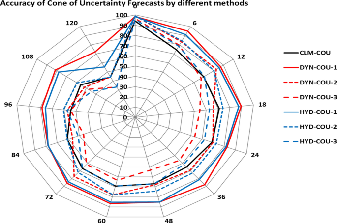
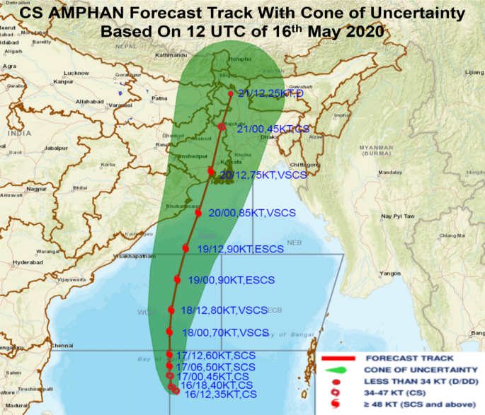
The resulting visualization clearly shows the point forecast surrounded by a shaded region representing the 95% prediction interval. This interval provides critical context: in periods of high volatility, the band widens, signaling greater uncertainty. In more stable periods, it narrows. This visual information is invaluable for a business user, transforming a simple forecast into a sophisticated risk assessment tool.
Section 3: Implications and Insights for Real-World Applications
The shift from point to probabilistic forecasting is more than a technical curiosity; it has profound implications for how businesses operate and make decisions. By quantifying uncertainty, organizations can move from reactive to proactive strategies.
Probabilistic forecast chart with uncertainty bands – Deterministic and probabilistic flood forecasting for 20050902 …
From Guesswork to Strategic Buffering
Consider an e-commerce company managing inventory. A point forecast might predict 1,000 units of a product will be sold next month. Should the company stock exactly 1,000 units? Doing so risks a stockout if demand is higher, leading to lost sales and customer dissatisfaction. A probabilistic forecast, however, might reveal a 95% prediction interval of [850, 1150] units. This information empowers the inventory manager to make a strategic decision. They could stock 1,150 units to be 97.5% confident they won’t run out, or choose a level of 1,100 units to balance the cost of holding inventory against the risk of a stockout. This transforms inventory management from guesswork into a data-driven risk optimization problem.
Enhancing Financial Risk Management
In finance, forecasting asset prices, revenue, or costs with only point estimates is notoriously risky. Probabilistic forecasts provide a framework for stress testing and scenario analysis. A financial planner can use the prediction intervals for future revenue to assess the likelihood of meeting debt obligations or funding new projects. For example, if the lower bound of the 90% confidence interval for next quarter’s revenue falls below the operational cost, it serves as an early warning signal to secure additional financing or cut expenses. This is a far more robust approach than relying on a single “most likely” scenario.
Building Trust and Transparency
One of the less-discussed benefits of providing prediction intervals is building trust with stakeholders. Presenting a single number can seem overly confident and can erode credibility when the prediction is inevitably wrong. By presenting a range, data scientists are transparently communicating the limits of their model’s knowledge. This honesty fosters a more sophisticated and realistic conversation about the future, where discussions center on managing a range of possible outcomes rather than arguing about the accuracy of a single predicted number.
Section 4: Best Practices, Pitfalls, and Recommendations
While powerful, implementing these techniques requires care and attention to detail. Adhering to best practices is key to generating reliable and meaningful results.
Stock market prediction chart – Workflow of a stock market prediction model with supervised …
Pros and Cons
Pros:
Statistical Guarantees: Conformal Prediction provides distribution-free coverage guarantees, making it highly reliable.
Model-Agnostic: It can be applied to virtually any regression model, offering immense flexibility.
Interpretability: The output (a prediction range) is intuitive for business stakeholders.
Efficiency: When paired with fast models like randomized networks, it can be computationally very efficient.
Cons:
Data Requirement: It requires a dedicated calibration set, reducing the amount of data available for training.
Interval Width: If the underlying model is poor or the data is inherently noisy, the prediction intervals can become too wide to be useful. The quality of the interval depends on the quality of the point forecast.
Assumption of Exchangeability: The core theory assumes that the data points (train, calibration, and test) are exchangeable (drawn from the same distribution). This can be violated in time series with significant concept drift.
Recommendations and Tips
Handle Data Drift: In time series, the underlying patterns can change over time. It’s often best to use a more recent block of data for calibration and testing to ensure the model’s error estimates are relevant to the near future.
Choose Alpha Wisely: The confidence level (1 – alpha) is a business decision. A 99% interval will be wider and safer but less precise, while an 80% interval will be narrower but riskier. Align this choice with the specific application’s risk tolerance.
Start Simple: The model-agnostic nature of Conformal Prediction means you can start with a simple, fast baseline model (like Ridge or LightGBM) before moving to more complex architectures. The insights gained from a simple model are often just as valuable.
Monitor Interval Width: Keep track of the average width of your prediction intervals over time. A consistently widening interval can be an early indicator that your model needs to be retrained due to data drift.
Conclusion
The landscape of time series forecasting is undergoing a fundamental and exciting evolution. The latest python news from the machine learning community signals a clear move away from the limitations of single-point predictions and toward the richer, more informative world of probabilistic forecasting. By combining computationally efficient models with robust uncertainty quantification frameworks like Conformal Prediction, data scientists can now deliver not just a prediction, but a comprehensive view of future possibilities.
This approach provides statistically sound prediction intervals that empower businesses to make smarter, risk-aware decisions in areas from supply chain management to financial planning. As open-source Python libraries like mapie continue to make these advanced techniques more accessible, the ability to quantify and communicate uncertainty will no longer be a niche capability but a standard expectation for any serious forecasting task. Embracing this paradigm shift is key to unlocking the next level of value from time series data.
