Mastering Python Finance: From Data Gathering to Advanced Algorithmic Trading Strategies

The financial technology landscape has undergone a seismic shift over the last decade, transitioning from spreadsheet-dominated workflows to sophisticated, code-driven ecosystems. At the heart of this revolution is Python finance. As the de facto language for data science and algorithmic trading, Python provides the glue between raw market data and actionable investment strategies. Whether you are a quantitative analyst, a developer building a fintech startup, or a trader looking to automate execution, understanding the full lifecycle of financial data analysis is paramount.

In this comprehensive guide, we will explore the modern Python financial stack. We will move beyond basic scripting to explore high-performance data handling with the Polars dataframe library, leverage DuckDB python for efficient querying, and discuss how modern tooling like the Uv installer and Rye manager are reshaping project management. Furthermore, we will touch upon cutting-edge developments such as GIL removal (Free threading) in CPython internals and how Local LLM integration via LangChain updates is changing how we interpret unstructured financial data.

Section 1: Modern Data Gathering and Management

The first step in any quantitative workflow is acquiring high-quality data. In the past, this often meant downloading CSVs manually. Today, we rely on robust APIs and web scraping. While libraries like yfinance remain popular for prototyping, production-grade systems require more resilience. With Scrapy updates and Playwright python, developers can now scrape alternative data—such as sentiment from news sites or retail pricing data—to gain an edge.

Efficient Storage with DuckDB and PyArrow

Once data is ingested, storage efficiency becomes critical. Traditional CSV files are slow and cumbersome. The modern approach utilizes PyArrow updates to handle data in the Parquet format, which is columnar and highly compressed. To query this data without loading it entirely into RAM, DuckDB python has emerged as a game-changer. It allows for SQL queries directly on Parquet files, acting as an in-process analytical database.

Furthermore, the Ibis framework allows you to write Pythonic code that translates to SQL, decoupling your logic from the underlying engine. This is essential when scaling from a local laptop to a cloud data warehouse.

import yfinance as yf
import duckdb
import pandas as pd
from datetime import datetime, timedelta

def fetch_and_store_data(tickers, period="5y"):
    """
    Fetches data using yfinance and stores it efficiently using DuckDB.
    """
    print(f"Fetching data for: {tickers}")
    
    # Download data
    data = yf.download(tickers, period=period, group_by='ticker', auto_adjust=True)
    
    # Reshape data for database storage (Long format)
    frames = []
    for ticker in tickers:
        df = data[ticker].copy()
        df['Ticker'] = ticker
        df.reset_index(inplace=True)
        frames.append(df)
        
    combined_df = pd.concat(frames)
    
    # Rename columns to be SQL friendly
    combined_df.columns = [c.lower().replace(' ', '_') for c in combined_df.columns]
    
    # Initialize DuckDB connection
    con = duckdb.connect('financial_data.db')
    
    # Store data directly from the DataFrame into a DuckDB table
    # efficient upsert logic would go here in production
    con.execute("CREATE TABLE IF NOT EXISTS stock_prices AS SELECT * FROM combined_df")
    con.execute("INSERT INTO stock_prices SELECT * FROM combined_df")
    
    print("Data stored successfully in DuckDB.")
    
    # Example Analytical Query: Calculate average volume per ticker
    result = con.execute("""
        SELECT ticker, AVG(volume) as avg_vol 
        FROM stock_prices 
        GROUP BY ticker 
        ORDER BY avg_vol DESC
    """).df()
    
    con.close()
    return result

# Usage
if __name__ == "__main__":
    top_tech = ["AAPL", "MSFT", "NVDA", "GOOGL"]
    summary = fetch_and_store_data(top_tech)
    print(summary)

Section 2: High-Performance Analysis and Strategy Implementation

Once the data is secured, the focus shifts to analysis. For years, Pandas has been the king. However, with Pandas updates and NumPy news continuing to roll out, a challenger has appeared: Polars. Polars is written in Rust and utilizes the Apache Arrow memory format. It is multi-threaded by default, contrasting with the single-threaded nature of standard Pandas operations.

Leveraging Rust Python and GIL Removal

The intersection of Rust Python tools (like Polars and Ruff) is significantly accelerating financial computing. Additionally, the Python community is buzzing about the GIL removal (Global Interpreter Lock) in upcoming Python versions (Free threading). This is a monumental shift for algo trading backtesters, which often require heavy CPU computation for Monte Carlo simulations or optimization tasks. Until fully mainstream, libraries like Polars bridge the gap by executing logic outside the Python GIL.

Below is an example of calculating technical indicators using Polars. Notice the syntax similarity to Pandas but with a focus on expression contexts for speed.

import polars as pl
import numpy as np

def calculate_technical_indicators(parquet_path):
    """
    Loads data using Polars and calculates RSI and SMA efficiently.
    """
    # Scan parquet allows lazy evaluation - highly efficient for large datasets
    q = (
        pl.scan_parquet(parquet_path)
        .sort("date")
        .group_by("ticker")
        .map_groups(lambda df: df.with_columns([
            # Calculate Simple Moving Average (SMA)
            pl.col("close").rolling_mean(window_size=20).alias("sma_20"),
            
            # Calculate Daily Returns
            pl.col("close").pct_change().alias("daily_return"),
        ]))
    )
    
    # Execute the lazy query
    df = q.collect()
    
    # Custom RSI Calculation using Polars expressions
    # RSI requires a bit more logic than a simple rolling mean
    def calculate_rsi(series, period=14):
        delta = series.diff()
        gain = delta.clip(lower_bound=0)
        loss = -delta.clip(upper_bound=0)
        
        avg_gain = gain.rolling_mean(window_size=period)
        avg_loss = loss.rolling_mean(window_size=period)
        
        rs = avg_gain / avg_loss
        return 100 - (100 / (1 + rs))

    # Apply RSI
    df = df.with_columns(
        pl.col("close").map_batches(lambda s: calculate_rsi(s)).alias("rsi_14")
    )
    
    # Filter for potential buy signals (Strategy Logic)
    # Condition: Price above SMA20 AND RSI < 30 (Oversold)
    signals = df.filter(
        (pl.col("close") > pl.col("sma_20")) & 
        (pl.col("rsi_14") < 30)
    )
    
    return signals

# Note: In a real scenario, you would point this to the parquet file generated in Section 1
# signals = calculate_technical_indicators("financial_data.parquet")

Section 3: Advanced Techniques - AI, ML, and Automation

Python finance is no longer just about moving averages. The integration of Machine Learning and Large Language Models (LLMs) is defining the next generation of strategies. With Scikit-learn updates improving regression models and PyTorch news highlighting better support for time-series forecasting (like LSTMs or Transformers), the toolkit is vast.

Sentiment Analysis with Local LLMs

One of the most exciting areas is analyzing unstructured data (earnings call transcripts, news headlines). Using LangChain updates and LlamaIndex news, developers can build RAG (Retrieval-Augmented Generation) pipelines. By running a Local LLM (like Llama 3 or Mistral) via tools like Ollama or HuggingFace, financial institutions can process sensitive data on-premise without sending it to external APIs, addressing Python security concerns.

Furthermore, we are seeing the nascence of Python quantum computing in finance. Qiskit news suggests that quantum algorithms for portfolio optimization are moving from theoretical to experimental phases, offering speeds impossible with classical computers.

Here is how you might structure a prediction pipeline using a Random Forest Classifier, a staple in Keras updates and Scikit-learn workflows for its robustness against overfitting compared to deep neural networks on noisy financial data.

from sklearn.ensemble import RandomForestClassifier
from sklearn.model_selection import train_test_split
from sklearn.metrics import precision_score
import pandas as pd

def build_prediction_model(df):
    """
    Builds a machine learning model to predict market direction.
    """
    # Feature Engineering
    df['Target'] = (df['close'].shift(-1) > df['close']).astype(int) # 1 if next day is higher
    
    features = ['close', 'volume', 'open', 'high', 'low']
    
    # Drop NaNs created by lagging/shifting
    df.dropna(inplace=True)
    
    X = df[features]
    y = df['Target']
    
    # Split data (Time-series split is better, but using random for simplicity here)
    # In finance, ALWAYS split by time (train on past, test on future)
    split = int(len(df) * 0.8)
    X_train, X_test = X.iloc[:split], X.iloc[split:]
    y_train, y_test = y.iloc[:split], y.iloc[split:]
    
    # Initialize Model
    # n_estimators and min_samples_split help reduce overfitting
    model = RandomForestClassifier(n_estimators=100, min_samples_split=10, random_state=42)
    
    # Train
    model.fit(X_train, y_train)
    
    # Predict
    preds = model.predict(X_test)
    
    # Evaluate
    precision = precision_score(y_test, preds)
    print(f"Model Precision: {precision:.4f}")
    
    return model

# This function assumes 'df' is a Pandas DataFrame populated with market data

Section 4: Best Practices, Tooling, and Deployment

Writing the code is only half the battle. Managing the ecosystem is where projects often fail. The Python packaging landscape is evolving rapidly. The Uv installer and Rye manager are setting new standards for speed and dependency resolution, replacing slower workflows involving pure pip or poetry. Additionally, using the Hatch build system or PDM manager ensures your project is reproducible.

Code Quality and Security

In finance, a bug can cost millions. Therefore, rigorous testing and linting are non-negotiable. Ruff linter has taken the community by storm due to its speed (written in Rust), replacing Flake8 and isort for many. Combined with the Black formatter, your code style remains consistent. Static analysis using Type hints and MyPy updates helps catch type-related errors before runtime. For security, tools like SonarLint python and checks for Malware analysis in dependencies (via PyPI safety audits) are essential to prevent supply chain attacks.

Modern Web UI and APIs

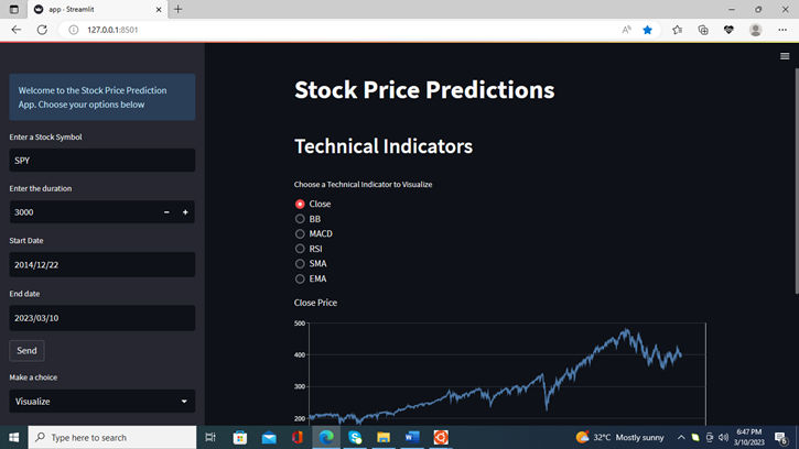
To visualize strategies, developers are moving away from static plots. FastAPI news highlights its dominance for building high-performance asynchronous APIs to serve model predictions. For the frontend, pure Python frameworks like Reflex app, Flet ui, and Taipy news allow data scientists to build interactive dashboards without knowing JavaScript. PyScript web technology even allows Python to run directly in the browser via WebAssembly.

Below is a modern project configuration example using a FastAPI skeleton that utilizes type hinting and async capabilities.

from fastapi import FastAPI, HTTPException
from pydantic import BaseModel
from typing import List, Optional
import uvicorn

# Define data models using Pydantic (Type hints)
class StockRequest(BaseModel):
    ticker: str
    lookback_days: int = 30

class PredictionResponse(BaseModel):
    ticker: str
    predicted_direction: str
    confidence: float

app = FastAPI(title="QuantAlgo API", description="API for serving ML predictions")

@app.get("/")
async def root():
    return {"message": "Financial Algo API is running"}

@app.post("/predict", response_model=PredictionResponse)
async def get_prediction(request: StockRequest):
    """
    Endpoint to get a prediction for a specific stock.
    """
    # Simulate processing time or DB lookup
    if request.ticker not in ["AAPL", "GOOG", "TSLA"]:
        raise HTTPException(status_code=404, detail="Ticker not supported in model")
    
    # In a real app, load the model (from Section 3) and infer
    # Here we mock the response
    return PredictionResponse(
        ticker=request.ticker,
        predicted_direction="UP",
        confidence=0.78
    )

# To run: uvicorn main:app --reload
# This leverages Starlette and Pydantic for high-speed async performance

Conclusion

The journey from data gathering to advanced analysis in Python finance is evolving at a breakneck pace. We have moved from simple CSV parsing to complex pipelines involving DuckDB, Polars, and Local LLM integration. The ecosystem is becoming faster with Rust Python tools and safer with strict typing and modern linters like Ruff.

Looking ahead, technologies like the Mojo language promise to bring C-level performance with Python syntax, potentially revolutionizing high-frequency trading. Meanwhile, Edge AI and Python automation will continue to democratize institutional-grade analytics for individual developers. To stay ahead, focus on mastering the modern stack—efficient data storage, vectorized analysis, and robust deployment pipelines. The future of finance is code, and Python is the key.